Problem 1a: L2-norm geometric margin minimization formulation of Var-SVM
for {solver_exp} = {CAR}, {VAN}, {BULDOZER}, {TANK}
minimize quadratic
subject to
var_risk
linearmulti
solver: solver_exp, precision = 9, stages = 30
end for
——————————————————————–
quadratic = quadratic function specified by a unit matrix
var_risk = Value-at-Risk specified by a matrix of scenarios
linearmulti = set of linear functions specified by a matrix of scenarios
——————————————————————–
Data and solution in Run-File Environment

Problem Datasets				# of Variables	# of Scenarios	Objective Value (BULDOZER)	Solving Time (BULDOZER), PC 2.66GHz (sec)
Dataset1	Problem Statement	Data	Solution	2	100	18.702062913380	0.22
Dataset2	Problem Statement	Data	Solution	3	100	4.012808007875	0.25

Problem 1b: L2-norm structural risk minimization formulation of Var-SVM
for {solver_exp} = {CAR}, {VAN}, {BULDOZER}, {TANK}
minimize quadratic + var
subject to
linearmulti
solver: solver_exp, precision = 9, stages = 30
end for
——————————————————————–
quadratic = quadratic function specified by a unit matrix
var_risk = Value-at-Risk specified by a matrix of scenarios
linearmulti = set of linear functions specified by a matrix of scenarios
——————————————————————–
Data and solution in Run-File Environment

Problem Datasets				# of Variables	# of Scenarios	Objective Value (BULDOZER)	Solving Time (BULDOZER), PC 2.66GHz (sec)
Dataset1	Problem Statement	Data	Solution	2	100	-0.013367514210	0.22
Dataset2	Problem Statement	Data	Solution	3	100	-0.062300476773	0.25

Problem 2a: L1-norm geometric margin minimization formulation of Var-SVM
for {solver_exp} = {CAR}, {VAN}, {BULDOZER}, {TANK}
minimize polynom_abs
subject to
var_risk
linearmulti
solver: solver_exp, precision = 9, stages = 30
end for
——————————————————————–
polynom_abs = L1-norm function
var_risk = Value-at-Risk specified by a matrix of scenarios
linearmulti = set of linear functions specified by a matrix of scenarios
——————————————————————–
Data and solution in Run-File Environment

Problem Datasets				# of Variables	# of Scenarios	Objective Value (BULDOZER)	Solving Time (BULDOZER), PC 2.66GHz (sec)
Dataset1	Problem Statement	Data	Solution	2	100	6.115910927534	0.07
Dataset2	Problem Statement	Data	Solution	3	100	4.100144111911	0.24

Problem 2b: L1-norm structural risk minimization formulation of Var-SVM
for {solver_exp} = {CAR}, {VAN}, {BULDOZER}, {TANK}
minimize polynom_abs + var_risk
subject to
linearmulti
solver: solver_exp, precision = 9, stages = 30
end for
——————————————————————–
polynom_abs = L1-norm function
var_risk = Value-at-Risk specified by a matrix of scenarios
linearmulti = set of linear functions specified by a matrix of scenarios
——————————————————————–
Data and solution in Run-File Environment

Problem Datasets				# of Variables	# of Scenarios	Objective Value (BULDOZER)	Solving Time (BULDOZER), PC 2.66GHz (sec)
Dataset1	Problem Statement	Data	Solution	2	100	-8.259128038970	0.28
Dataset2	Problem Statement	Data	Solution	3	100	-26.654598309919	0.27

CASE STUDY SUMMARY
This case study compares performance of several software packages for finding a solution to the Value-at-Risk Support Vector Machine (Var-SVM) classification problem. Given a training dataset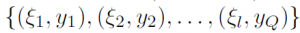 , consisting of Q points with feature vectors 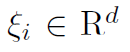and class labels 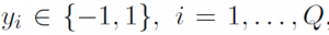, an SVM classification problem is to build a hyperplain 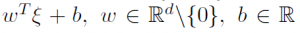in the feature space, that maximizes the geometric margin between the classes and the hyperplain. The original SVM was introduced by Vapnik [1979] for the case of maximization of an L2-norm margin and further reduced to a convex quadratic programming problem (QP) as long as the data set was separable. Nowadays, this formulation is known as a hard-margin SVM. In the case of a non-separable data set Cortes and Vapnik [1995] introduced the so-called soft-margin SVM, which can be viewed as a structural risk minimization problem, i.e., as a trade-off between an empirical classication error term and a regularization term, which is added to control overtting. Tsyurmasto et al. [2013] considers a generalization of the maximum margin approach corresponding to a particular choice of an empirical risk functional and provides a set of examples for such generalizations including hard- and soft-margin SVMs and nu-SVM. They also show, that for a positive homogeneous empirical risk functional both maximum margin and minimum structural risk L2-norm formulations provide the same solution, i.e., the same separating hyperplane. Zdanovskaya et al. [2014] provide an extension of this result for the case of L1-norm. Tsyurmasto et al. [2014] proposed a Var-SVM which corresponds to a positive homogeneous Value-at-Risk (VaR) empirical risk function. The main advantage of the Var-SVM is that it is stable to data outliers. The main disadvantage of the Var-SVM is that the problem is nonconvex and therefore is hard to solve. In this case study we consider four different formulations of Var-SVMs: 1a) maximum margin in L1-norm formulation, 1b) minimum structural risk in L1-norm formulation, 2a) maximum margin in L2-norm formulation, 2b) minimum structural risk in L2-norm formulation. To find a heuristic solution of the above Var-SVMs we use Portfolio Safeguard (PSG), since it has a preprogrammed Value-at-Risk function (VaR). In order to find an optimal solution of the above Var-SVMs we employ a mixed-integer linear programming representation (MILP representation) of VaR empirical risk functional proposed in Zdanovskaya et al. [2014]. This MILP representation is known to be NP-hard (see Benati and Rizzi [2007]). We further use such commercial solvers as Gurobi and Xpress to solve the derived Var-SVMs problems via the Branch&Bound algorithm. Our computational experiments show, that it may take Gurobi and Xpress up to several hours to find an optimal solution of Var-SVMs even for small datasets. Whereas it takes less than a second for PSG to find a corresponding heuristic solution.

References

Stefano Benati and Romeo Rizzi. A mixed integer linear programming formulation of the optimal mean/value-at-risk portfolio problem. European Journal of Operational Research, 176(1):423-434, 2007.

Corinna Cortes and Vladimir Vapnik. Support-vector networks. Machine learning, 20(3):273-297, 1995.

Nicklas Larsen, Helmut Mausser, and Stanislav Uryasev. Algorithms for optimization of value-at-risk. In Panos M. Pardalos and Vassilis K. Tsitsiringos, editors, Financial Engineering, E-commerce and Supply Chain, volume 70 of Applied Optimization, pages 19-46. Springer US, 2002.

Peter Tsyurmasto, J Gotoh, and S Uryasev. Support vector classication with positive homogeneous risk functionals. Technical report, Research Report 2013-4, Department of Industrial and Systems Engineering, University of Florida.(Downloadable from www.ise.ufl.edu/uryasev/publications), 2013.

Peter Tsyurmasto, Michael Zabarankin, and Stan Uryasev. Value-at-risk support vector machine: stability to outliers. Journal of Combinatorial Optimization, 28(1):218-232, 2014.

Vladimir Vapnik. Estimation of Dependences Based on Empirical Data [in Russian]. Nauka, Moscow, 1979. (English translation: Springer Verlag, New York, 1982).

Victoria Zdanovskaya, Konstantin Pavlikov, and Stan Uryasev. Value-at-risk support vector machine: Mixed integer programming formulation and equivalence of problem statements, 2014.